This is an ongoing project designed to use data from the University of Glasgow’s experiment entitled ‘Video recording true single-photon double-slit interference’ (http://researchdata.gla.ac.uk/281/) and to compare the results of that experiment to the predicted results generated by the time dependent Schrödinger equation.
The code can be split into three sections:
1) Importing, cleaning and visualizing the data from the real double slit experiment.
2) Simulating the situation using the Schrodinger equation.
3) Comparing that real data to the simulation, identifying any deviation.
Section 1: Importing, Cleaning and Visualizing
The first step was importing the data. The data was supplied in the ASCII format and saved as .asc files. The data stream is a series of numbers with 0s representing non-collisions and numbers above 0 representing where collisions have occurred with the detector. While the data stream is just a flat series of binary, the data itself was collected by a 512 x 512 camera. As such it needed to be placed into a numPy matrix of 512×512. It was then converted into a dataframe and displayed as a heatmap with the Viridis colour theme as imaged below:
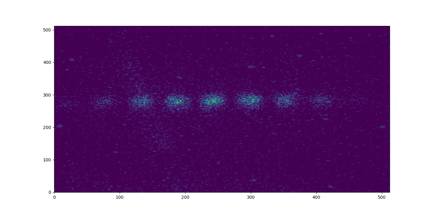
The above image is after 40012 photons had been fired at the detector. The green areas show where collisions have occurred, the lighter the green the more collisions that have occurred. The areas coloured in matte purple are where no collisions have occurred.
The following is the first attempt I have made of visualizing the collisions in a video file. Note that the video has been sped up with th eintention of making it more watchable, and therefore does not include every particle collision piecemeal. For it to have included every collision 1-by-1 the video would have needed to be 33 minutes and 55 seconds long.
Section 2: The Simulation
The hard part. Ongoing so is not yet complete but feel free to read on to get an idea of where I am going.
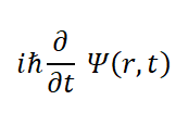
The dynamics of quantum mechanics in most situations are given by the time-dependent Schrödinger equation:
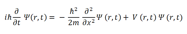
The equation is not intuitive, but it does follow the general format of total energy of the system on the left with the Hamiltonian (kinetic energy + potential energy) on the right of the equals sign.
Let’s break down this equation a little starting with the Hamiltonian. First there is the kinetic energy of the system:
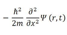
where:
i is an imaginary number, √-1
ħ is planck’s reduced constant, or planck’s constant divide 2π, which equals 1.05459 x 10⁻³⁴ joule-second.
r is a real coordinate space, for one dimension this is {x}, for two {x,y}, for three {x,y,z}.
t is time
∂ and ∂t etc,
∂2/∂x2, is the laplacian operator this will sometimes be represented with ∇2. ??? Check this x, pretty sure it should be an r. damn it. ???
m is mass of the particle
Ψ is a sinusoidal wave function designed to represent a Gaussian/normal distribution.
Then there is the potential energy of the system:
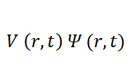
where:
i is an imaginary number
ħ is planck’s reduced constant
Ψ is a sinusoidal function designed to represent a Gaussian/normal distribution.
When these two components are added together they result in the total energy of the system:
where:
i is an imaginary number
ħ is planck’s reduced constant
ψ is a sin function that is designed to represent a Gaussian distribution.
x is the location of the particle/object
t is the time progression
Fortunately, a lot of this code has already been completed by Jake Vanderplas and Andre Xuereb (https://github.com/jakevdp/pySchrodinger). However, for their version they restricted their system to 1 dimensional.
Note: The second dimension on the visualization of the Schrodinger equation is the probability amplitude, not a spatial dimension.
This means that any visualization of the Schrodinger equation will always have an extra probability dimension. A 2D visualization will be 3D, a 3D visualization will be 4D. Visualization in 4D is quite a trial, but has two potential options. The first is a 3D scatter plot and the second is series of 2D slices in a 3D space, with a heatmap in every slice.
Section 3: Simulation vs Experiment
Comparing. There are statistical tools to compare how much a given set of data deviates from normalcy. Given that the Schrodinger equation is a Gaussian distribution with a series of operators acting upon it the standard suite of tools to detect deviations from normalcy should apply.