This is my attempt to make property price predictions for the ‘House Prices: Advanced Regression Techniques’ competition on Kaggle (https://www.kaggle.com/c/house-prices-advanced-regression-techniques). It involves cleaning data, using regression techniques and fitting data to a machine learning model. The objective is to make increasingly accurate predictions of the prices in the test data set using the training data set.
There are four layers to this project:
1) Exploring the data
2) Cleaning the data
3) Featuring Engineering
4) Making Predictions/Model Fitting
Section 1: Exploring the data
Exploring the data is the first step as usual and in this case I used my own base template to perform some exploratory analysis. Check out the code below and read on for a bit more explanation:
trainVar.head() # Show first five rows of dataset
trainVar.describe() # Generate summary statistics
trainVar.shape # Describe rows x column counts
trainVar.keys() # Creates a list of column names, useful for feature searching.
trainVar.info() # Returns information of data types, columns, etc.
trainVar.columns # Shows a list of column names.
trainVar.corr() # Shows correlation between different variables on a scale of -1 to 1, where 0 is none ???
"""
The correlations section creates a descending list of correlations between
columns and the desired response variable (The thing we want to predict).
"""
correlations = train_df.corr() # convert train_df to a series of correlation values???
correlations = correlations["SalePrice"].sort_values(ascending=False) # Find correlation with SalePrice
features = correlations.index[1:6] # Why is this 1 to 6???
correlations

trainVar_null = pd.isnull(train_df).sum() # The number of null values in the training data.
testVar_null = pd.isnull(test_df).sum() # The number of null values in the test data.
The correlation heat map provides a correlation between the various variables. The code is as below:
#correlation map
f,ax = plt.subplots(figsize=(18, 18))
sns.heatmap(trainVar.corr(), annot=True, linewidths=.5, fmt= '.1f',ax=ax)
plt.show()
The outcome is the following heatmap:
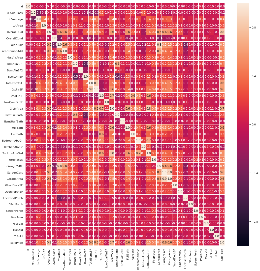
Now this might at a glance seem intimidating to look at, but it has a purpose. It shows us the relation between variables on a scale of -1 to 1 with -1 meaning perfect indirect correlation, 1 perfect correlation and 0 no correlation whatsoever. As a way to quickly get a look at data this approach is invaluable. It can give us clues as to what we should be looking for. In this particular case, however, we know we are interested only in the correlation between variables and the sale price so let’s have a closer look at the correlations with SalePrice using the following code:
"""
The correlations section creates a descending list of correlations between
columns and the desired response variable (The thing we want to predict).
"""
correlations = trainVar.corr() # convert train_df to a series of correlation values???
correlations = correlations["SalePrice"].sort_values(ascending=False) # Find correlation with SalePrice
features = correlations.index[1:6] # Why is this 1 to 6???
correlations
Which produces the following list of correlations ranked highest to lowest:
SalePrice 1.000000
OverallQual 0.790982
GrLivArea 0.708624
GarageCars 0.640409
GarageArea 0.623431
TotalBsmtSF 0.613581
1stFlrSF 0.605852
FullBath 0.560664
TotRmsAbvGrd 0.533723
YearBuilt 0.522897
YearRemodAdd 0.507101
GarageYrBlt 0.486362
MasVnrArea 0.477493
Fireplaces 0.466929
BsmtFinSF1 0.386420
LotFrontage 0.351799
WoodDeckSF 0.324413
2ndFlrSF 0.319334
OpenPorchSF 0.315856
HalfBath 0.284108
LotArea 0.263843
BsmtFullBath 0.227122
BsmtUnfSF 0.214479
BedroomAbvGr 0.168213
ScreenPorch 0.111447
PoolArea 0.092404
MoSold 0.046432
3SsnPorch 0.044584
BsmtFinSF2 -0.011378
BsmtHalfBath -0.016844
MiscVal -0.021190
Id -0.021917
LowQualFinSF -0.025606
YrSold -0.028923
OverallCond -0.077856
MSSubClass -0.084284
EnclosedPorch -0.128578
KitchenAbvGr -0.135907
Name: SalePrice, dtype: float64
Section 2: Cleaning the data
Section 3: Featuring Engineering
Section 4: Making Predictions/Model Fitting